Module 1 Project
Introduction
Now that we’ve been introduced to R and its important properties, lets now explore how this knowledge can be put to use in the context of data and a workflow more typical in organismal biology. For this project, we’ll be looking at scale puncture data from Prof. Kenaley’s lab. Briefly, these data come from experiments in which we used a motorized probe and force transducer to study how much force it takes to puncture fish scales from various locations on several species of fishes. The goal of analyzing these data is to assess if the magnitude of scale puncture resistance varies over the body and according to species. This data set is rather large (>1800 experiments!), but eminently suited for work in R (i.e., your head would spin trying to any of the following operations in Excel, say).
Set Up
Let’s first download these data as .csv file from this link. Don’t open the file in Excel or some other program. If your OS does so automatically, just close the file without making any changes. The file in most cases will be automatically downloaded to a “downloads” directory (i.e., folder). Copy or move this file to a new directory, perhaps one named “scales” in a folder for this and other BIOL 3140 projects.
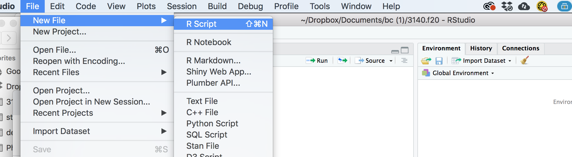
Open R Studio and create a new script (File->New->R script, see below). Save it (File->Save) with an appropriate title in your new “scales” directory.
To this new R script, let’s add our first lines of code. It’s a
general convention that we load the libraries of R packages that we want
to use in the R session (i.e., when R Studio is running R). Without
doing so, if you call functions that aren’t loaded in base R, you’ll
encounter an error. For this project and script, we need
ggplot, a handy plotting package and
tidyverse, a collection of data analysis packages. Make
sure you’ve installed them, something you should have done will reading
and working with HOPR. These initial lines of code would look like
this:
library(ggplot2)
library(tidyverse)
## ── Attaching core tidyverse packages ─────────────────
## ✔ dplyr 1.1.4 ✔ readr 2.1.5
## ✔ forcats 1.0.0 ✔ stringr 1.5.1
## ✔ lubridate 1.9.4 ✔ tibble 3.3.0
## ✔ purrr 1.0.4 ✔ tidyr 1.3.1
## ── Conflicts ──────────────── tidyverse_conflicts() ──
## ✖ dplyr::filter() masks stats::filter()
## ✖ dplyr::lag() masks stats::lag()
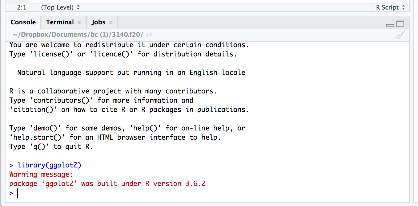
## ℹ Use the conflicted package (<http://conflicted.r-lib.org/>) to force all conflicts to become errorsGo ahead and just copy and paste these line into your script at line 1. Notice that when you do this nothing happens. Entering code, either by typing or pasting doesn’t tell R to run it. You must do so explicitly by selecting a section of code you want to run (the first line in this case) and pressing “enter” or compiling the entire script by clicking on the “run” icon at the top of the R Studio screen. Hit “run” and see what happens. In the console tab at the bottom of R Studio, you’ll see this:
The console is where you see what’s happening or has happened in the
R session. Go to the console and type in library(ggplot2)
and hit return. You’ve just asked R to load the ggplot2
library, but because it’s already loaded, you won’t get any red text in
response. Working in the console rather than running code line by line
in the script or compiling the whole script can be handy, especially
when you just want to do simple things that you don’t want saved in the
script. For instance, type 5000/3 into the console and hit
return. Notice you get your answer: 1666.667.
Let’s move on to another convention of writing an R script: setting the working directory. This is perhaps the most important step when working with external data in R (and doing so many other important tasks, like saving outputs from analyses, e.g., figures, tables, etc.). The working directory is a way of telling R where to find and save things. Without this input, R won’t know where to find or place important objects like data or figures, respectively.
setwd() is a command essential to working in R. It’s
hard to overstate just how important this component of a script is. As
we start using R projects (an integrated workflow in R and R Studio) and
R markdown (an authoring framework that combines text, code, and
graphics) in the course, the working directory gets set for you. But,
always keep in mind, someone or something must tell R where to look.
To perform this all important task, we’ll include a
setwd() command. This function merely needs a text string
that stipulates the path of the directory you want to work in. The path
may look something like, “~/Chris/Documents/bc/3140/scales”.
Note: This will be unique to almost everyone, that is,
we all have different naming conventions for our folders on our
computers. My name is Chris, I have a documents folder that contains a
“bc” directory, which contains a “3140” directory, which, in turn,
contains the “scales” directory I want to work in.
At first, typing in the text of a path may be confusing and less than
intuitive. If this is the case, there’s a hack. In R studio, just click
on “Session->Set Working Directory->Choose Directory” and, in the
file browser window, select the directory you want to work in (say
“scales” in this case) and press the “OPEN” icon. This will set the
working directory to “scales”. Notice that in the console, a
setwd() command has been entered and run, complete with the
file path. This file path will be the working directory for the script
until you change it through the same approach or close R Studio. When
you open your script in R Studio again, you’ll have to set the directory
again as well. To avoid this cumbersome step each time you start up R
and R Studio, just copy and paste the setwd() command from
the console into you script. Now your script should look something like
the following but with your own unique directory path to the working
directory:
library(ggplot2)
setwd("~/Chris/Documents/bc/3140/scales")
Select these lines in your script and run them or click on “run”. If all goes well you’ll see these lines appear in the console without any errors. If you made some error in typing in the file path, then you’ll get an error. For example, if I forget the trailing “s” in the “scales” part of the directory path as in this code, I would’ve gotten the following output:
library(ggplot2)
setwd("~/Chris/Documents/bc/3140/scale")
## Error in setwd("~/Chris/Documents/bc/3140/scale"): cannot change working directoryLoading Data
OK, now that we’ve gotten our working directory set, we can now load the “scales.csv” file that was placed in the “scales” directory.
dat <- read.csv("scales.csv")Here, the command read.csv() is used to read in the data
and the results are passed to the variable named dat, short
for data. By default, the results of reading in a .csv file with
read.csv() are stored as a data frame, a two dimensional
table-like object with rows and columns. Before we get to working with
these rows and columns, let’s first inspect what sort of data we have
and say something about what they mean.
One can see how large the data set is with dim() and
reveal the first few lines of the data with the function
head() :
dim(dat)## [1] 1842 4head(dat)## N quadrant species specimen
## 1 3.558803 UR A. rupestris Arup_1
## 2 3.528323 UR A. rupestris Arup_1
## 3 3.523567 UR A. rupestris Arup_1
## 4 2.988193 UR A. rupestris Arup_1
## 5 4.281844 UR A. rupestris Arup_1
## 6 4.955457 UR A. rupestris Arup_1Using the dim() function reveals that there are 1842
rows and 4 columns, while the head() command reveals that
there are columns named “N”, “quadrant”, “species”, and “specimen”. You
might simply want to run these lines in the console rather than from the
script—if this is in the script, each time you run it, you’ll get the
the dimensions and first 5 lines of the data printed to the console. You
really only need to do this once.
The 1842 rows represent the results of puncture experiments on that many scales. The four columns represent the following:
- “N” is the force (in Newtons) it took the needle to puncture a scale
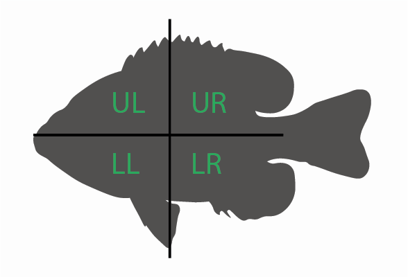
- “quadrant” indicates from where on the body the scale (see below):
- “UL”: Upper left of the body (anterodorsal quadrant)
- “UR”: Upper right of the body (posteroodorsal quadrant)
- “LL”: Lower right of the body (anteroventral quadrant)
- “LL”: Lower right of the body (posteroventral quadrant)
- “species” indicates from which species the scales came
- “specimen” indicates from which specimen the scales came (several for each species)
Now let’s see how these data are stored in R, that is, what class the
columns are. We can do this one of several ways using the function
class(). The first and most cumbersome would be to use the
subsetting techniques we’ve learning in HOPR to evaluate each column.
Remember that the $ symbol or numbers reflecting column
position (i.e., index) can be employed to retrieve specific columns.
Something like this:
#with "$"
class(dat$N)
## [1] "numeric"class(dat$quadrant)## [1] "character"class(dat$species)## [1] "character"class(dat$specimen)## [1] "character"#with index, produces the same result
class(dat[,1])## [1] "numeric"class(dat[,2])## [1] "character"class(dat[,3])## [1] "character"class(dat[,4])## [1] "character"Here, using either method, we see that the “N” column is numeric (it’s a continuous value corresponding to force), while all the other data columns contain factors, text strings to be exact, representing their discrete values for quadrant, species, and specimen. As you learned in HOPR, this means we must treat the numeric values differently than the factors and vice versa. Go ahead and try treating them the same:
mean(dat$N)## [1] 4.734429mean(dat$quadrant)## Warning in mean.default(dat$quadrant): argument is not numeric or logical:
## returning NA## [1] NANotice that R tells you that mean can’t be computed on “quadrant” because it is not numeric.
OK, so now we’ve learned what classes of data we have, but we’ve done
so in no fewer than four lines of code representing operations on each
of the columns. The power or R and other programming languages is that
there’s almost always a faster and simpler way of doing things. In this
case, we can inspect the class of out data in just one line using
sapply().
sapply(dat,class)## N quadrant species specimen
## "numeric" "character" "character" "character"Easy peasy with sapply(). Have a look at
?sapply(), the help entry, which explains that this
function applies another function over a vector. In the case of data
frames, sapply() applies a functions over a vector of
columns by default. This is considerably more tidy and speedy than
subsetting columns and repeating procedures over each.
Whenever you get an error in R, the tendency is to go right back to the code and try to fix things, paying little attention to the red text in the console. Errors often tell you something very important about your script and, in this example, your data. Be sure to read these errors carefully and makes sense of them before altering your code. Googling the error is often a huge help.
Simple Operations: Summarizing
Now that we know what sort of data and how much of it we have, let’s do some simple operations that a biologist might perform ahead of any analysis. Consider what additional and important things we want to know about our data. How many species are in our data set? How many specimens per species were included? How many observations (punctures) are there for each species? Yes, Yes, and Yes. These and other questions about the make up of your data can be answered through summarizations.
Let’s start with how many species we have. Because we’re working with
a character class for the species column, we first want to change that
to a factor. As we’ve learned from HOPR, factors have levels,i.e.,
unqique values. This is exaclty what we want: to find the unique values
for species. So let’s convert this column to a factor, then we can
inspect the levels. To change the column class to a factor and then
reveal the levels in factor-type data, we simply redefine the column and
then pass those data through levels:
dat$species <- as.factor(dat$species)
species <- levels(dat$species)
species
## [1] "A. rupestris" "L. gibbosus" "L. macrochirus" "Mi. salmoides"
## [5] "Mo. saxatilis" "P. flavescens"By storing the levels of species and calling “species” on separate
line, we see that there are 6 species in our data set. But let’s have R
tell us how many. We can count things in R with the
length() function:
length(species)## [1] 6The names and number of species, revealed in two lines of code. Pretty simple. Now how about how many observations per species. This is often a crucial piece of summary information, i.e., are there 1800 observations for A. rupestris and just a handful for all the others? If so, this wouldn’t be much of a comprehensive study across these species. Finding how many observations, as with previous operations, can be done in a number of different ways. And like these previous operations, let’s consider both cumbersome and more straightforward methods.
Because we have the levels (all unique values) of species stored,
let’s use that vector of names and some logical-test
operations we learned about in HOPR to subset the data frame and the
variable species and count the observations. Let’s take on
the first value of the species variable first. In the code
below, all the values in the species column are compared to the first
entry for “species” (“A. rupestris”) by using ==. This asks
the question Does the value to the left equal the value to the
right? In this specific case, we use == to ask Do
the values in dat$species equal the first value in the
“species” variable?
dat$species==species[1]Have a look at the result in the console (I’m not showing the output
here, because . . .). You should see hundreds of logical values,
TRUE and FALSE with many TRUE’s
at first. This indicates that the first 300 or so values for the
“species” column matches “A. rupestris”. Now we can nest these logical
values within the “species” vector (column) to return only those values
that match “A. rupestris”, like so:
dat$species[dat$species==species[1]]From here, we can find the length of this subsetted vector, save the
results in a new variable name that resembles that particular level of
“species”, and then iterate through all the levels of “species”. After
this, let’s combine the results in a data frame using our
species variable and c() to combine our new
length variables.
A.rup<-length(dat$species[dat$species==species[1]])
L.gib<-length(dat$species[dat$species==species[2]])
L.mac<-length(dat$species[dat$species==species[3]])
M.sal<-length(dat$species[dat$species==species[4]])
M.sax<-length(dat$species[dat$species==species[5]])
P.fla<-length(dat$species[dat$species==species[6]])

#combine the results with species
species.obs <- data.frame(sp=species,n=c(A.rup,L.gib,L.mac,M.sal,M.sax,P.fla))
species.obs
## sp n
## 1 A. rupestris 363
## 2 L. gibbosus 252
## 3 L. macrochirus 368
## 4 Mi. salmoides 310
## 5 Mo. saxatilis 289
## 6 P. flavescens 260There we have it, the number of observations/punctures for each species. Pretty evenly distributed, so not to worry about widely uneven sample sizes. This is great, but, this took many lines of code and some “hard coding”, that is, explicitly inputting a value. The hard coding issue here is with typing in the numeric potion (“1”, “2”, “3”, etc.) for each entry in our “species” variable. This is a drag and opens the door to mistakes. Why not let R do the iterations for you?
As we’re learning, summarizing data is an important step in any analysis. Fortunately, succinct methods and operations in R for summarizing exist in several popular packages. Perhaps the most widely used are those curated in “tidyverse”, a set of R packages designed for data science. All the packages in tidyverse share an underlying design philosophy, grammar (what the functions looks like and ask for), and data structures, making it a one stop shopping experience for data analysis. We’ll introduce how to summarize data using functions from tidyverse here and move on to more involved operations using tidyverse in the next module. Should should already have tidyverse installed and loaded.
tidyverse includes the dplyr package, a super helpful
library of functions for data analysis. Let’s use its
summarise() and group_by() functions and pipe
convention (%>%) to find the number of punctures per
species. The summarise() function creates variables that
summarize the data according to variables of interest. We set these
variables of interest using group_by(). The pipe,
%>%, is used to combine data with these functions. As
we’ll see in more detail later, the pipe %>% passes
results from left to right. Using the pipe with the data and the
functions group_by() and summarize(), we
summarize our data by species rather succinctly.
dat %>%
  group_by(species) %>%
  summarise(n = n())
## # A tibble: 6 × 2
## species n
## <fct> <int>
## 1 A. rupestris 363
## 2 L. gibbosus 252
## 3 L. macrochirus 368
## 4 Mi. salmoides 310
## 5 Mo. saxatilis 289
## 6 P. flavescens 260What this code essentially means is pass the data through the
function group_by(), grouping it by the “species” column,
and summarize it according to group with a count, n().
Notice the result is a tibble, a particular type of data object, akin to
a data frame. We’ll discuss tibbles more in the next module.
Of course, we can save these results to a variable.
species.n<- dat %>%
  group_by(species) %>%
  summarise(n = n())
species.n
## # A tibble: 6 × 2
## species n
## <fct> <int>
## 1 A. rupestris 363
## 2 L. gibbosus 252
## 3 L. macrochirus 368
## 4 Mi. salmoides 310
## 5 Mo. saxatilis 289
## 6 P. flavescens 260Now we haven’t answered one of our questions, How many specimens
for each species?. This, again is super easy with
dplyr and the pipe. Here, we pass our data to a
count() function that counts observations according to
groups (“species” and “specimen” in this case), use print()
so you can see the output, and then we count this output of observations
by “species” to find the unique values of “specimen”.
dat %>%
  count(species,specimen) %>%
  print() %>%
  count(species,name = "n.specimens")
## species specimen n
## 1 A. rupestris Arup_1 100
## 2 A. rupestris Arup_2 83
## 3 A. rupestris Arup_3 78
## 4 A. rupestris Arup_4 102
## 5 L. gibbosus Lgib_1 52
## 6 L. gibbosus Lgib_2 53
## 7 L. gibbosus Lgib_3 53
## 8 L. gibbosus Lgib_4 55
## 9 L. gibbosus Lgib_5 39
## 10 L. macrochirus Lmac_1 115
## 11 L. macrochirus Lmac_2 74
## 12 L. macrochirus Lmac_3 58
## 13 L. macrochirus Lmac_4 61
## 14 L. macrochirus Lmac_5 60
## 15 Mi. salmoides Msal_1 136
## 16 Mi. salmoides Msal_2 57
## 17 Mi. salmoides Msal_3 76
## 18 Mi. salmoides Msal_4 41
## 19 Mo. saxatilis Msax_1 100
## 20 Mo. saxatilis Msax_2 97
## 21 Mo. saxatilis Msax_3 92
## 22 P. flavescens Pfla_1 83
## 23 P. flavescens Pfla_2 62
## 24 P. flavescens Pfla_3 66
## 25 P. flavescens Pfla_4 49## species n.specimens
## 1 A. rupestris 4
## 2 L. gibbosus 5
## 3 L. macrochirus 5
## 4 Mi. salmoides 4
## 5 Mo. saxatilis 3
## 6 P. flavescens 4By now, you’re head may be spinning like a top. This is a lot to take in. Don’t worry! We’re just running quickly through the basics and won’t worry too much about committing any of this to memory. Just keep moving through this project, logging these operations in your R script, and you can always come back to specific parts when challenged by similar tasks in the future.
Loop When You Can
Phew! You’re almost there, the end of the Module 1 Project. Just one
last important concept to work through, the loop, specifically, the
for loop. This is a great device for iterating through
operations for which there aren’t dedicated functions. Important
examples of this in the context of organismal biology include loading
data from many files into one data set and producing a bunch of figures
all at once from a large data set, among other things. Since we have a
large data set loaded, why don’t we use a for() loop to
produce a bunch of figures.
A for() loop essentially tells R to do something over a
set of things in a vector. For instance, for “i” in 1 to 10, print each
“i”:
for(i in 1:10) print(i)## [1] 1
## [1] 2
## [1] 3
## [1] 4
## [1] 5
## [1] 6
## [1] 7
## [1] 8
## [1] 9
## [1] 10In the context of doing something much more complicated, this saves a
bunch of time. Back to our example of saving many figures from our large
data set. Consider the case of plotting the mean puncture force for each
quadrant in each species. This is easily accomplished with a short
for() loop that works over our species
variable and contains a filter, pipes, and a ggplot()
operation.
for(i in species){
  p <- dat %>%
  filter(species==i)%>%
 ggplot()+geom_boxplot(aes(x=quadrant,y=N))+ggtitle(i)
 print(p)
}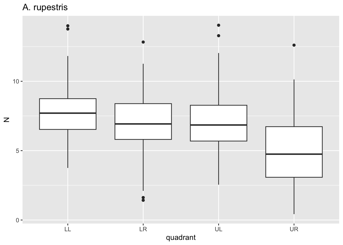
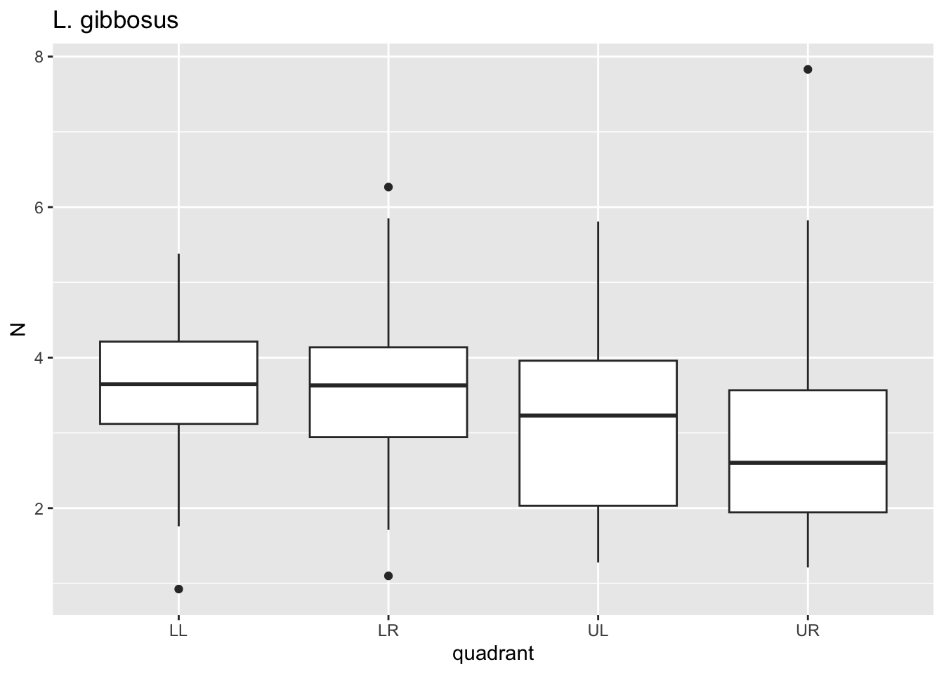
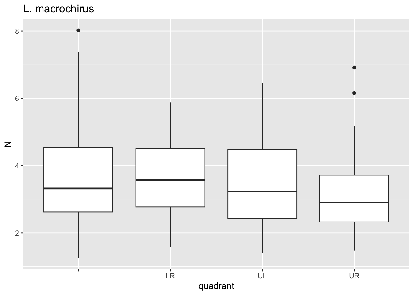
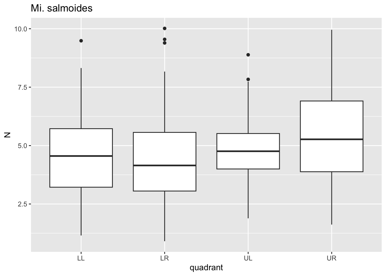
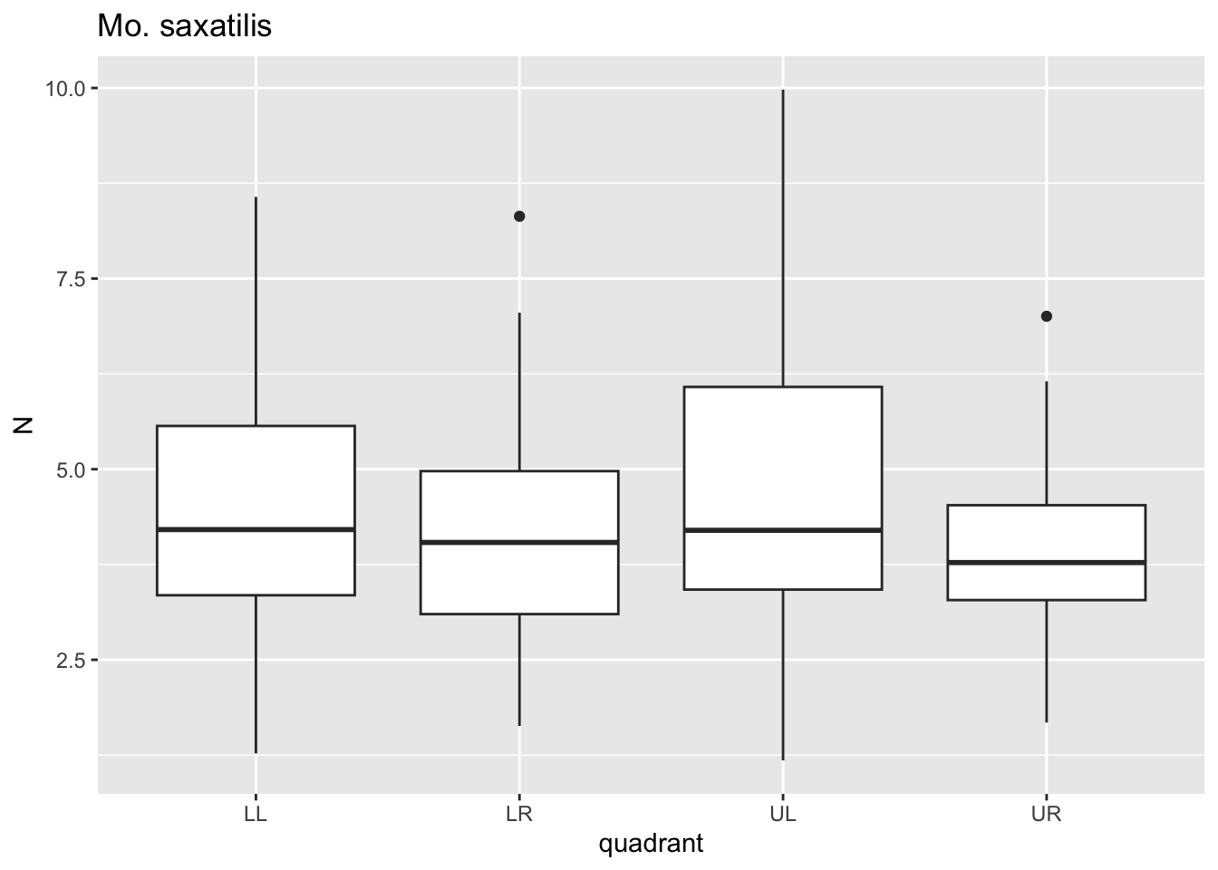
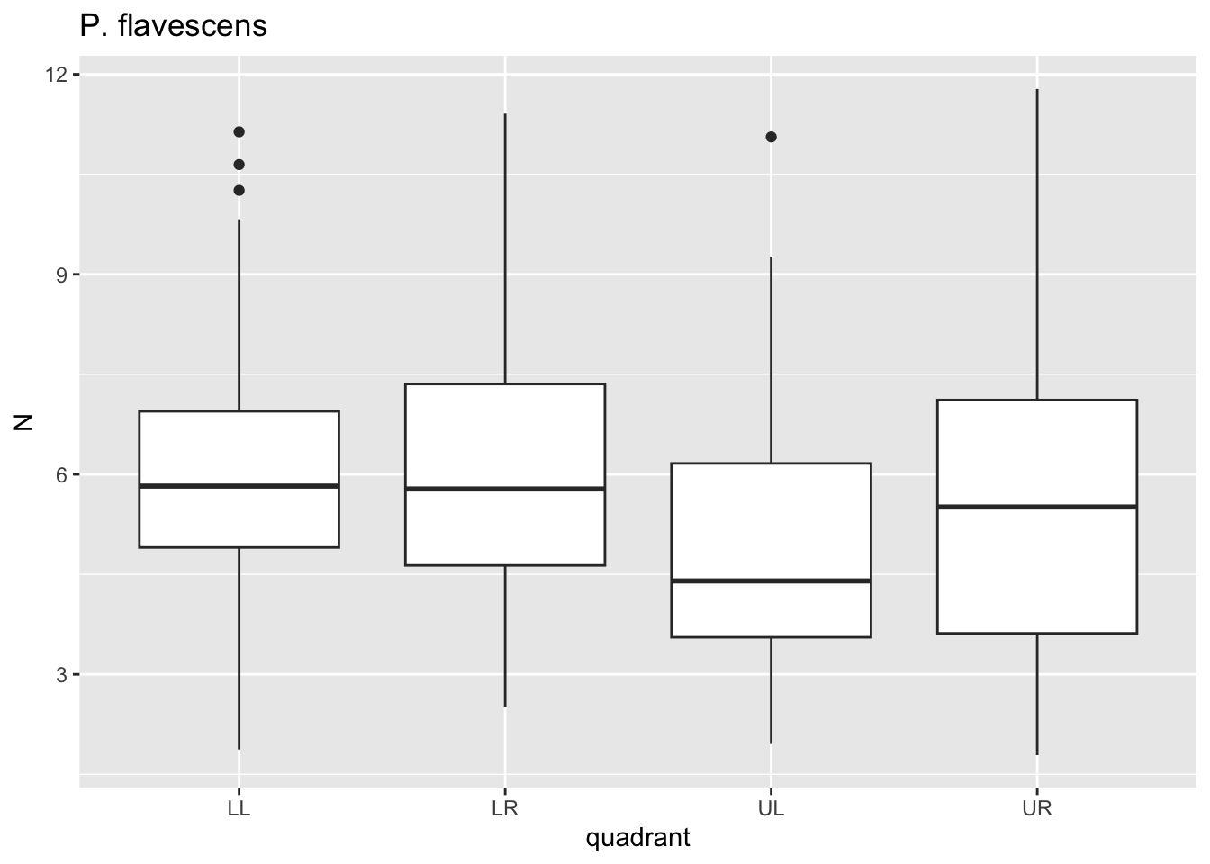
Here, for each value i in species we passed
dat through a filter where species==i, plotted
a boxplot using ggplot where x is the quadrant, y is the
puncture force. For each species, this got saved to p and
then we printed p. Notice that 6 separate plots are sent
sequentially to the “Plots” tab in the lower right panel. This is where
graphical results are shown in R Studio. No need to establish 6 separate
pieces of code for each figure.
Let’s wrap this up by saving a PDF file containing all the figures.
pdf("species_quadrant.pdf")
for(i in species){
  p <- dat %>%
  filter(species==i)%>%
 ggplot()+geom_boxplot(aes(x=quadrant,y=N))+ggtitle(i)
 print(p)
}
dev.off()
## quartz_off_screen
## 2list.files(pattern=".pdf")## [1] "DeVries_etal_20210.pdf" "Mortolaetal.pdf" "shark_points.pdf"
## [4] "species_quadrant.pdf" "species.quadrant.pdf"The wrapping function pdf() prints graphic output to a
file, in this case one named “species_quadrant.pdf”. Any plot printed
with p() after pdf() and before
dev.off() saves the plots in the named file. The
list.files() command with pattern=".pdf"
confirms that a PDF file was saved to our working directory.
Project Report
The goal of this project report is to submit an R script that runs the code presented above and produces the PDF of mean puncture force across each quadrant for each species. For the project to be complete, the script must include the following:
- A
datvariable containing the scales dataset. - A line of code which reports the class of each column in the dataset.
- A line of code which reports the dimensions of the dataset.
- Code that produces a summary of the number of scales punctured for each species.
- Code that produces a summary of the number of specimens sampled for each species.
- Code that produces a PDF file containing 6 figures, one for each species that includes a boxplot of puncture force verus quadrant.
- A commented section of text that serves as the AI-use statement.
Each team member must submit their own report. Make sure each commits their code and PDF to your team’s repo, appropriately named, e.g., “Jane_Doe_script.R”, “Jane_Doe_species_quandrant.pdf”. This means each team member should push their submission to their team’s github directory, i.e., “Module1_Team1”, if in Team 1. Submissions are due by 11:59 PM on Sunday, September 7th.