Introduction

White-tailed deer (WTD, Odocoileus virginianus) are native to much of North America and represent an ecologically important species across a diverse array of habitats, from dense mixed forest to open farm- and grasslands. The currently estimated WTD population of 30 million in the United States is about the same as pre-colonization. Due to a combination of over hunting and poor resource management practices, the US population dipped to fewer than 2 million by about 1900, but the abundance of this species has been on a steady rebound for over the last 100 years.

However, the historical abundance of WTD in New England is largely different from the continental trend. New England marks the northern edge of the species’ historical range and WTD were rare in the area, especially in northern New England. What’s more, due to post-colonial land-use practices—particularly, near total deforestation for agricultural purposes–WTD were largely extirpated from the area by the late 18th century. With changes associated with a move away from an agrarian economy, reforestation, and the succession of mixed habitats, WTD abundance slowly increased through the last half of the 20th century. However, it’s only recently, say within the last few decades, that New England WTD abundance has increased sharply, particularly in suburban areas.

The question of what’s driven this recent sharp increase in WTD abundance is the focus of this project. In particular, we’ll ask:

Is there spatial heterogeneity in WTD harvest (number taken during hunting season, a proxy for abundance)
If so, is spatial heterogeneity in WTD harvest associated with land-use patterns.

For this we’ll focus on the great state of New Hampshire, Prof. Kenaley’s birthplace.

To answer such a question, one could, of course, assemble harvest and land-use data for the Granite State as a whole and commence with the typical statistical operations (e.g., linear modeling, a la harvest~population*land-use). However, NH is a rather diverse state in the form, potentially predictive variable. In the north of the state, there are lots of forests. In the southern part of the state, there a lots more people, and a mix of developed, forested, and agricultural land. In between, we have a diversity of land uses, included forested, farmed, and forgotten (i.e., successional) areas. That is, each of these attributes vary spatially across the landscape and focusing on this great state as a whole wouldn’t account for the important variation across it. We therefore need to enter the realm of spatial analysis, specifically spatial association. By this, we mean the degree to which things are similarly arranged in space.

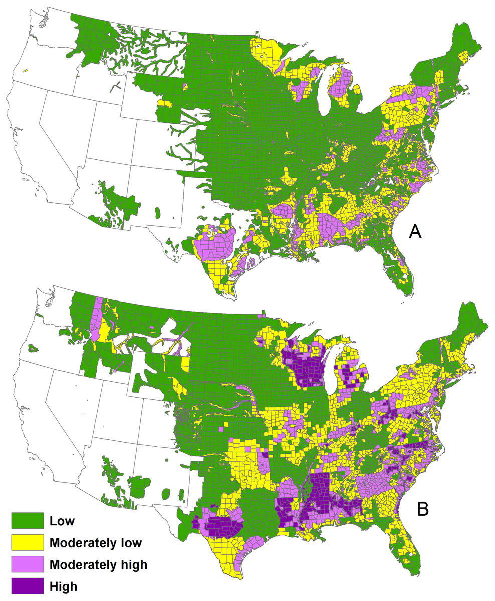
The 1982 WTD densities (A) and 2001–2005 deer densities (B) in the continental United States.

Just a few decades ago, to assess such a spatial question would require buying extremely expensive pieces of software.

Let’s take a momentary break from the icy climes of the granite state and consider how spatial analysis might be undertaken in R. We’ll consider examples from a much more beachy place, Bermuda, where, as far as I know, there are no WTD.

Spatial Analysis in R

Many R packages have been developed for spatial analysis. Many are idiosyncratic, requiring one to work with particular object classes that don’t work well with other data-science frameworks like tidyverse. There are a few, namely sf and stars that do work well with the tidyverse. sf provides a table format for simple features, a spatial object class where feature geometries are stored in a list-column (i.e., each row contains a column as a list of shape geometries). stars was written by several of the same sf authors to support raster data among other things (e.g., time series). The development of both packages came from the bottom up, with lots of input from the data science community that relies so much on tidyverse. The packages are designed to work together. Functions or methods operating on sf or stars objects start with st_, making it easy to recognize them as appropriate for spatial tasks in the sf and stars workflow.

The Spatial Analysis Framework

Spatial analysis is a sprawling field in data science. Although spatial data and its analysis is often simply treated as longitude and latitude and some attribute or variable that varies with it, the field is so much more. Yes, coordinates are important, but so are the patterns that emerge when we consider how attributes vary within and between spatial areas and grids.

This representation of data in shape or grid format marks an important framework within spatial analysis: in addition to point (coordinate) data, attributes are often aggregated within either shapes (e.g., lines, polygons, etc.) or grids. The former is considered shape information, the later raster information, an allusion to pixels of an image. We can obtain shape or raster data from myriad sources: state and federal agencies, universities and non-profit organizations, and even R packages that facilitate data download.

Working with shape data

Shape data often contain geopolitical information (e.g.,city, state, or country boundaries) and even topological data (e.g., the boundaries of rivers, lakes, and oceans, and elevation contours). For instance, let’s load a shape of the beautiful country of Bermuda using the rnauturalearth package and kick up sf, the package of choice that deals in shape data, to produce a simple map:

library(rnaturalearth)
library(sf)

## Linking to GEOS 3.11.0, GDAL 3.5.3, PROJ 9.1.0; sf_use_s2() is TRUE

library(tidyverse)

## Warning: package 'ggplot2' was built under R version 4.2.3

## ── Attaching core tidyverse packages ──────────────────────── tidyverse 2.0.0 ──
## ✔ dplyr     1.1.1     ✔ readr     2.1.4
## ✔ forcats   1.0.0     ✔ stringr   1.5.0
## ✔ ggplot2   3.5.1     ✔ tibble    3.2.1
## ✔ lubridate 1.9.2     ✔ tidyr     1.3.0
## ✔ purrr     1.0.1

## ── Conflicts ────────────────────────────────────────── tidyverse_conflicts() ──
## ✖ dplyr::filter() masks stats::filter()
## ✖ dplyr::lag()    masks stats::lag()
## ℹ Use the conflicted package (<http://conflicted.r-lib.org/>) to force all conflicts to become errors

bermuda <- ne_states(country="Bermuda") %>% 
   st_as_sf

bermuda %>% 
  ggplot()+
  geom_sf()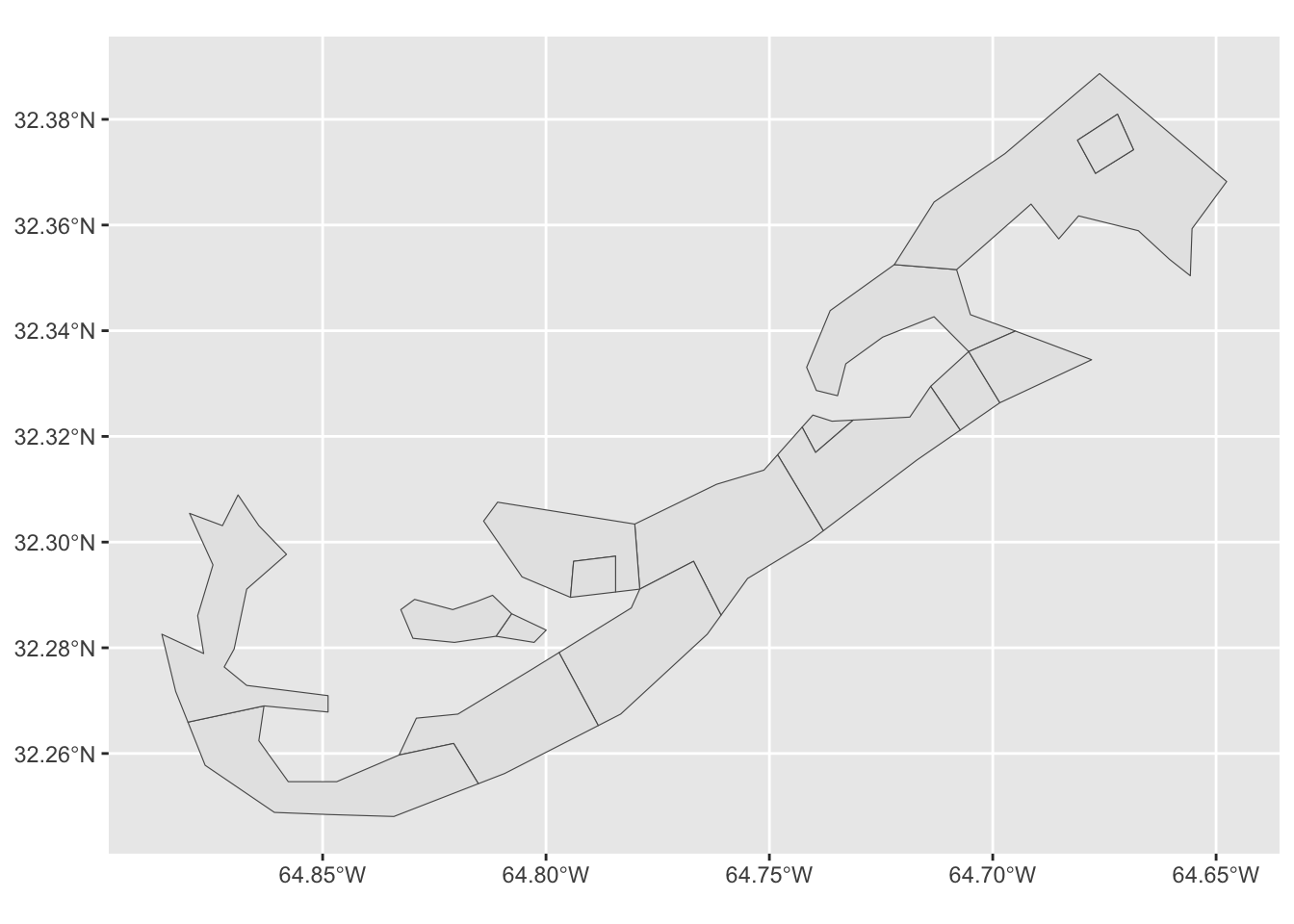

Notice here, that we have to convert the shape retrieved from the rnaturalearth package (an object of class “SpatialPolygonsDataFrame”) to an sf object. This sort of conversion is perhaps the most vexing part of spatial analysis in R. That is, many spatial object classes exist depending on the R package used and to work with objects across functions of different origins, conversion needs to happen. Yet, we’re often unsure of which conversion function to use. We’ll try to keep conversion to a minimum in this project, but be ware. Fortunately, sf has the handy st_as_sf() that allows conversion of a spatial polygon data frame to an sf object.

Because sf plays nice with the tidyverse, to plot an sf object, we can use the ggplot() framework that’s become so much of the class. For this we use sf’s geom_sf().

Working with raster data

Raster data is presented in essentially pixel format. That is, each pixel in a spatial field represents 3 dimensions: some area of a particular 2D resolution (e.g., 30 x 30 m, 1 x 1 km) and some value of an attribute, like the color of an image.

Say for instance, we wanted to know the spatial distribution of population in Bermuda in 2020 at a resolution of 1 x 1 km, we could load a raster set from the worldpop.org, an organization devoted to distributing such data. For this, we’ll depend on the R raster powerhouse package, stars

library(stars)

## Loading required package: abind

bermuda_pop <- read_stars("https://data.worldpop.org/GIS/Population_Density/Global_2000_2020_1km/2020/BMU/bmu_pd_2020_1km.tif") %>% st_crop(bermuda)


  ggplot()+
  geom_stars(data=bermuda_pop)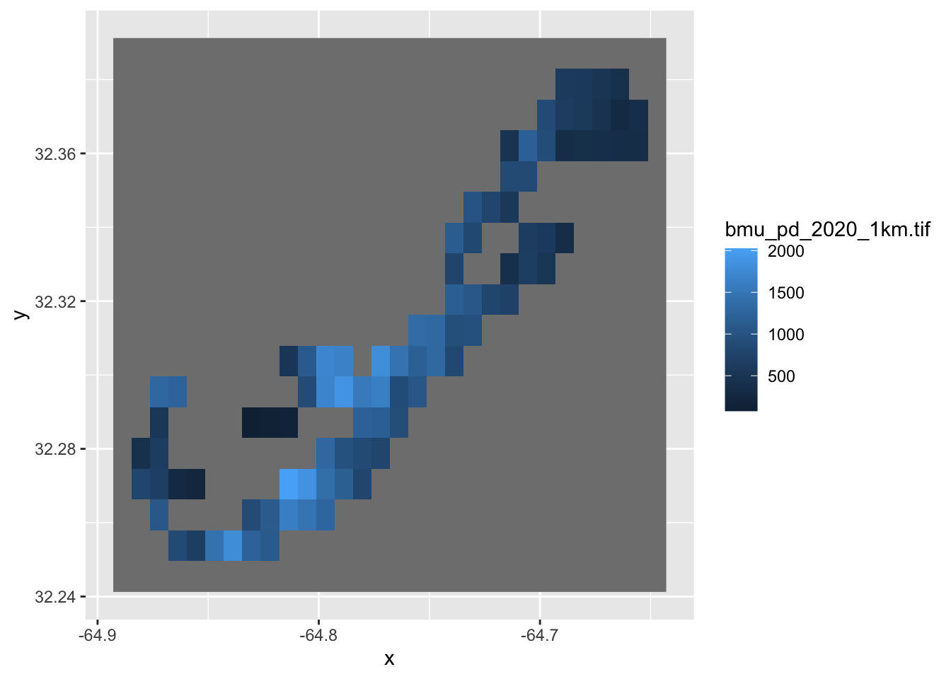

Here, we load the 1-km raster using read_stars() and cropped the data to the extent of our shape map using st_crop(). Plotting is simple as, like with sf, stars was designed to work well with tidyverse and ggplot. Here, we can make use of geom_stars() to plot a stars object in ggplot. Notice that, because Bermuda is a small island, the 1 km resolution is rather coarse.

Combining shape and raster data

Now, say we wanted to visually assess how these population tiles vary with the parish geopolitical boundaries in the the Bermuda map. For this, we need to combine the shape and population data and calculate the total population in each parish. We can start with the bermuda_pop stars object and then:

set the name of the first (and only) layer to an intuitive name, “population”, with setNames()
convert the stars object to an sf object with st_as_sf()
join the bermuda shape data to this, now sf, object with sf_join. This nests the raster (i.e., population) data within the extents of shapes (i.e., parishes) data
use dplyr’s group_by() to group by the parish (name)
and finally, sum the population based on this grouping.

What’s left to do is plot with geom_sf() as before with the bermuda sf object. Note that we add some bells and whistles to make in prettier.

bermuda2 <-  bermuda_pop %>% 
  setNames("population") %>% 
  st_as_sf() %>% 
  st_join( bermuda) %>% 
  group_by(name) %>% 
  summarise(population=sum(population))

bermuda %>% 
  ggplot() +
  geom_sf()+
  geom_sf(data=bermuda2,aes(fill=population))+
  geom_sf_text(aes(label=name),alpha=0.3)+
  scale_fill_viridis_c(option="magma")

## Warning in st_point_on_surface.sfc(sf::st_zm(x)): st_point_on_surface may not
## give correct results for longitude/latitude data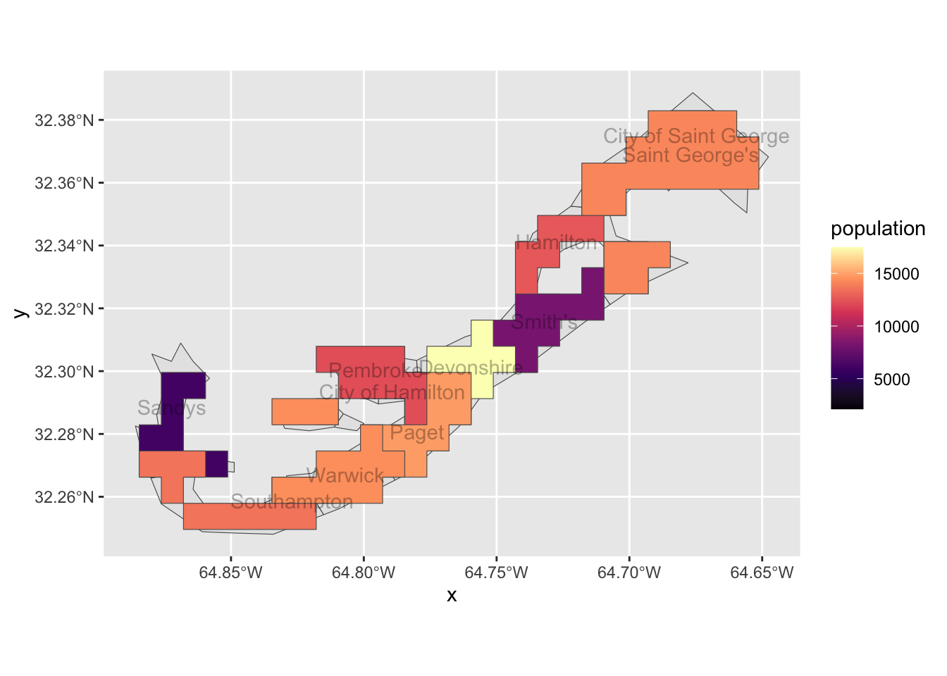

Lovely! We see that population does vary according to parish across the island, with Devonshire containing the highest population. Doing something like this will absolutely help us assess whether WTD varies spatially in New Hampshire. But, what might predict population density in Bermuda, an identical question to our second goal, of the project, i.e., does a variable (land-use patterns) predict WTD abundance. In our example of Bermuda, we lack such a predictive variable.We also lack any serious spatial resolution. That is, in the example above, we only consider 11 polygons.

For this, we’ll asses whether house color predicts population across the island as a much finer spatial scale.

House color varies a lot in Bermuda, but, by law, the roofs must be white as a means to keep homes cool.

Prof. Kenaley has assembled (eeeehhhem, simulated) house colors across the island according to sections of each parish, i.e. “subparish”, and created an sf shape file you can download here. Be sure to download and unzip the folder. I’ve done so to my “data” folder in my project directory so that the shape data are in “data/bermuda_shape”.

NOTE: shape files (ending in “.shp”) must have a bit of associated metadata files (e.g.,“.proj”,“.shx”,“.dbf”) in their directory to be loaded correctly. Make sure these are there.

So let’s use the sf function read_sf() to read in the shape file and have a look at the sf object that was loaded.

bermuda_house <- read_sf("data/bermuda_shape/bermuda_dat.shp") 

head(bermuda_house)

## Simple feature collection with 6 features and 10 fields
## Geometry type: POLYGON
## Dimension:     XY
## Bounding box:  xmin: -64.79452 ymin: 32.28955 xmax: -64.67599 ymax: 32.37808
## Geodetic CRS:  WGS 84
## # A tibble: 6 × 11
##   name       subparish tot_pop pred_col   blue green orange   pink purple  white
##   <chr>      <chr>       <dbl> <chr>     <dbl> <dbl>  <dbl>  <dbl>  <dbl>  <dbl>
## 1 City of H… subparis…    1243 green    0.0428 0.310 0.203  0.0535 0.257  0.134 
## 2 City of H… subparis…    1348 green    0.314  0.366 0.0825 0.0722 0.0876 0.0773
## 3 City of H… subparis…    1208 green    0.253  0.353 0.0706 0.0941 0.218  0.0118
## 4 City of H… subparis…    1212 green    0.0848 0.255 0.0667 0.206  0.145  0.242 
## 5 City of H… subparis…    1271 green    0.156  0.252 0.0816 0.245  0.163  0.102 
## 6 City of S… subparis…     208 orange   0.0385 0.231 0.346  0.0769 0.115  0.192 
## # ℹ 1 more variable: geometry <POLYGON [°]>

Note that we have several columns of interest. Namely:

name: the name of the parish
subparish: the subparish
tot_pop: the total population in each subparish (i.e., roughly the parish population/length(subparish))
pred_col: the predominant color in each subparish.
blue, green, orange, pink, purple and white: the proportion of each house color in the subparish.
lastly, the geometry: the polygon list that circumscribes each subparish.

Let’s have a look at what these data all mean spatially by plotting. Note that color has been set manually to match those of the pred_col column.

bermuda_house %>% 
  ggplot()+
  geom_sf(aes(fill=pred_col),alpha=0.5) +
    scale_fill_manual(values=c("blue","green","orange","pink","purple","grey90"))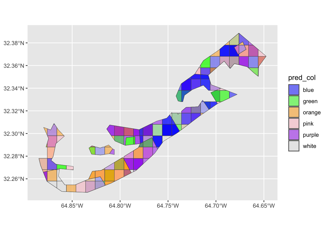

As we can see, the predominant color varies spatially. We now have a reasonable spatial data set to commence with some formal statistical analysis. How to move ahead with analysis, grasshopper, is a very interesting problem indeed.

Walking through random forests

You’ll notice that in the bermuda_house sf object, we have relative proportions of each house color for each subparish in addition to the predominant house color (pred_color). Indeed, the former was calculated from the latter. Plotting these quickly, it looks like there is some general pattern in the data across the island. How we should assess these patterns according to it’s spatial reach is the problem at hand.

bermuda_house %>% 
  ggplot(aes(pred_col,log(tot_pop),fill=pred_col))+
  geom_boxplot(alpha=0.5)+
    scale_fill_manual(values=c("blue","green","orange","pink","purple","grey90"))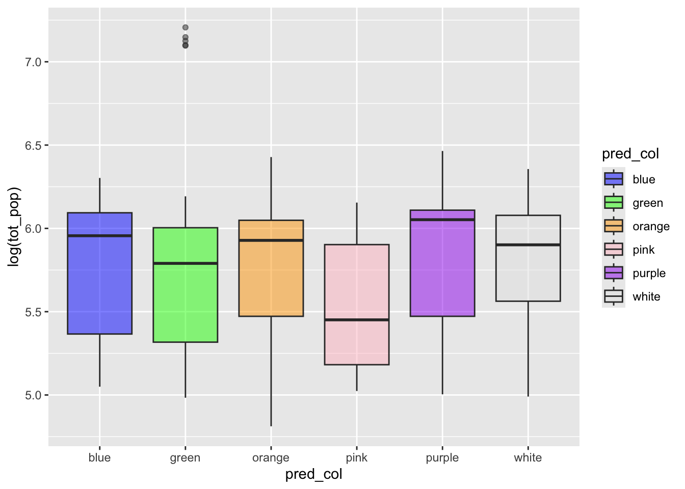

bermuda_house %>% 
  pivot_longer(blue:white,names_to = "color") %>% 
  ggplot(aes(value,log(tot_pop)))+
  geom_point()+
  geom_smooth(method="lm")+
  facet_wrap(.~color)

## `geom_smooth()` using formula = 'y ~ x'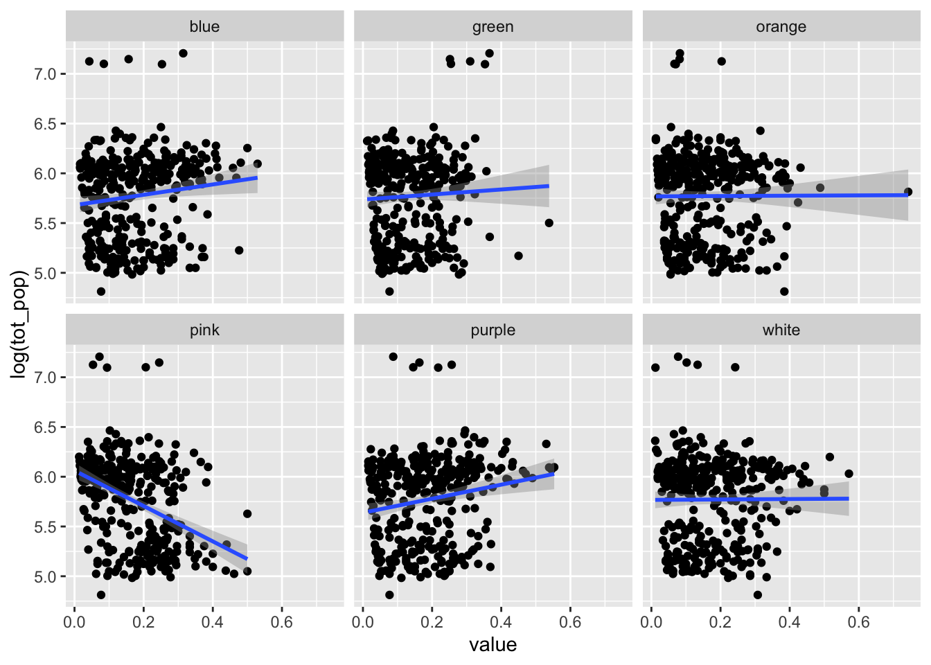

Many statistical approaches to spatial analysis exist. Of course, the approach we choose must be appropriate to the data.

In our case, each variable has its pros and cons. pred_col is a factor, a discrete variable with a finite set of levels (i.e. “blue”, “white”, etc.). One could use a logistical regression approach, but this is fraught and discrete predictors are rarely the only variable in the predictive mix. As for the proportion data with it’s >2 categories, one could use multinomial logistic or Dirichlet regression. There are paths for this in R, but again, they are fraught.

We also have another problem, one much deeper and unrelated to the statistical approaches mentioned above. Over space, any attribute value at any location is more likely to be similar to a value at an adjacent or close location than it is to a value from a distant location. That is, spatial data are often spatially autocorrelated. This violates a major assumption in many statistical models that the data/observations be independent.

So, what to do? Fortunately, we can leverage an evermore popular approach to estimating predictions from highly correlated data: Random Forests, a relatively straight forward machine learning algorithm.

Random forest is a supervised learning algorithm that incorporates three basic principles: decision trees, ensemble learning, and bootstrapping.

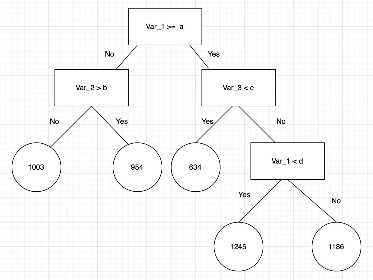
Decision trees. These are decision paths in which binary choices are made. In RF regression, decision trees start at a root and follow splits based on variable outcomes until a leaf node is reached and the result is given. The figure above represents the concept of a single decision tree which starts with the variable “Var_1” and splits based off of specific criteria. When “yes”, the decision tree follows the represented path, when ‘no’, the decision tree goes down the other path. This process repeats until the decision tree reaches the leaf node and the resulting outcome is decided. In RF regression, the values of a, b, c, or d could be any numeric value.

Ensemble learning. This is the process of using multiple models built (i.e, trained) over the same data. Model results are averaged to estimate a prediction. For an ensemble prediction to be powerful and accurate, the errors of each model (in this case decision tree) must be independent and different from tree to tree.

Bootstrapping. This is the process of randomly sampling subsets of a data set over a given number of iterations and a given number of variables and repeating an analysis based on each resample of the data. Results of each analysis are then averaged together to obtain a more powerful result than one analysis alone. Bootstrapping is a common ensemble method to infer emergent patterns in data science and the method upon which data for RF decision trees are generated.

RF regression models are powerful and accurate. They usually perform well on many problems, including features with non-linear relationships (our problem!!). Disadvantages, however, include the that there often hard to interpret (though only kinda), overfitting may easily occur, and one must choose the number of variables to bootstrap and the number of trees to include in the model.

Let’s see how we can put this into action using the R package randomForest. First, let’ load the package and assemble the data.

library(randomForest)

rf_dat <-  bermuda_house %>%
  ungroup %>%
  st_drop_geometry() %>%  
  na.omit  %>%  
  dplyr::select(-name,-pred_col,-subparish)

head(rf_dat)

## # A tibble: 6 × 7
##   tot_pop   blue green orange   pink purple  white
##     <dbl>  <dbl> <dbl>  <dbl>  <dbl>  <dbl>  <dbl>
## 1    1243 0.0428 0.310 0.203  0.0535 0.257  0.134 
## 2    1348 0.314  0.366 0.0825 0.0722 0.0876 0.0773
## 3    1208 0.253  0.353 0.0706 0.0941 0.218  0.0118
## 4    1212 0.0848 0.255 0.0667 0.206  0.145  0.242 
## 5    1271 0.156  0.252 0.0816 0.245  0.163  0.102 
## 6     208 0.0385 0.231 0.346  0.0769 0.115  0.192

Here we simply dropped the geometry list column with st_drop_geometry(), omitted any NA values, and removed the other columns we don’t need.

To run a random forest regression model with randomForest, one needs to specify a model formula, the number of trees to construct, and the number of variables to randomly sample at each split (i.e., node) in the trees. Here we say we want tot_pop to be predicted by all the other variables (i.e., proportion of each house color) with tot_pop~. mtry, the number of variables to sample at the splits is set to 2 and the number of trees (ntree) to 1000. Note that we also set importance=T to calculate the importance of each predictor, something we’ll use later.

rf <-randomForest(tot_pop~.,data=rf_dat, mtry=2, ntree=1000,importance=T,localImp=T)

Great, now we have an RF model that predicts population based on house color proportion. But, how do we interpret such a model? That is, what can the model tell us? The most logical approach would be to assess if the model made reasonable predictions and then, assess what variables contribute most to the patterns of populations across the subparishes. This, together, would answer our original question, does house color predict population?

Let’s first address if the model made an accurate prediction across all the subparishes. The function randomForest() returns the predicted values. So let’s add them to our rf_dat object and compare them to the actual population in each subparish with a plot.

#add predicitons
rf_dat$pred_pop<- rf$predicted


rf_dat %>% 
  mutate_at(c("tot_pop","pred_pop"),log) %>% 
  ggplot(aes(tot_pop,pred_pop))+
  geom_point()+
  geom_smooth(method="lm")

## `geom_smooth()` using formula = 'y ~ x'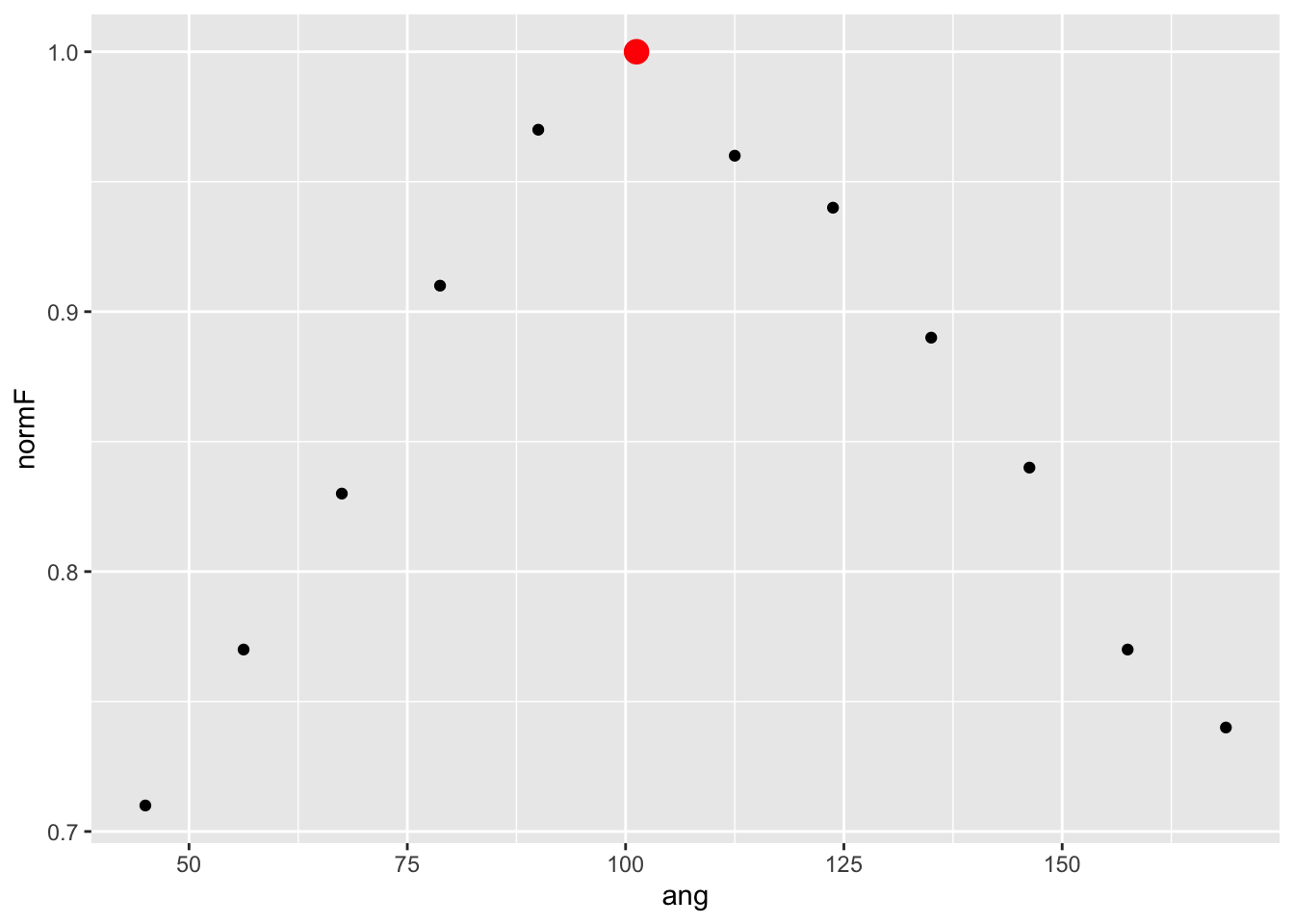

Looks as though the predictions were somewhat accurate. Now, what variables were important in making these accurate predictions? randForest has a basic function to assess this: varImpPlot(). So let’s run this on our model.

varImpPlot(rf,type=1)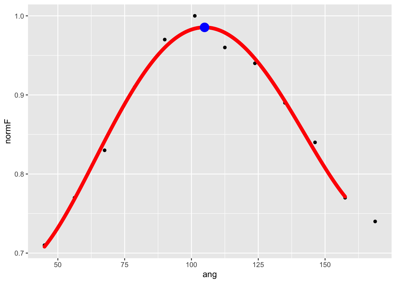

Here, we’re interested in the %IncMSE value (from type=1, see ?importance). This is pretty wonky, so bare with. For each tree, each predictor in the sample is randomly chosen in the bootstrap and passed through the tree to obtain an error rate (mean square error–MSE) in the regression. The error rate from the unchosen variables is then subtracted from the error rate of the chosen trees, and averaged across all trees. When this value is large, it implies that a variable is highly correlated to the dependent variable. In short, this tells us blue and pink houses predict population best. And thus, we have answered our question.

OK, this superb. But, as mentioned above, one tricky aspect of RF models is that we have to specify values for important parameters, namely mtry and the number of trees.

Let’s first look at the effect of number of trees. If we plot the rf model object, what’s returned is a trace of the model error as more trees were added to the sample. Note that ntree was set to 1000 and by tree 300, the error has stabilized. So it appears 1000 trees is enough.

plot(rf)

mtry-the number of variables to sample at each node in a tree-can have the most profound effect on the analysis. Let’s refine the model by tuning it according with the best value of mtry.

randomForest’s tuneRF() function permits quick and easy tuning assessment. One provides a starting value for mtry and an increment to change it by and the function performs the analysis changing mtry by this increment. It stops when there’s no more improvement in the error.

For example, what’s below starts with mtry = 1 and increases/decreases this value by a factor of 0.5 until the error stops improving by 1%. Note that tuneRF() requires a separate x and y value. As you can see, the optimal mtry value is 1. Perhaps the RF model should have been run with this value to start.

tuneRF(x=rf_dat %>% select(-tot_pop),
       y=rf_dat$tot_pop,
       stepFactor=0.5,
       ntreeTry=1000,
       trace=F,
       mtryStart = 1,
       improve = 0.01,
       )

## 0.005670609 0.01 
## 0.01079204 0.01

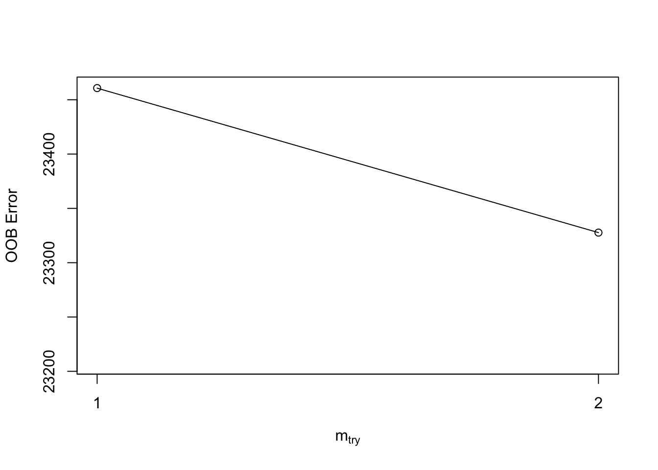
##   mtry OOBError
## 0    0 23207.55
## 1    1 23460.74
## 2    2 23327.70

Plotting prety maps in R

Lastly, let’s consider how to plot very nice trees in R. Many packages exist for this task, but perhaps none is more simple than the mapview package.

library(mapview)

mapview(bermuda_house, zcol = "pred_col")

Methods

Back to the frozen enclave of NH.

Using our Bermuda examples as a model, let’s perform a similar analysis. For this we’ll need harvest, geopolitical shape, and land-use data.

Harvest data source

OK, let’s first address the obvious. We will be using deer harvest data as a proxy for WTD abundance. Understandably, for some this may be a difficult thing with which to grapple. After all, we’re considering how many times a majestic animal has been killed, to put in plainly. There are many ethical considerations here and I’m happy to discuss them all in private. But, if we can, let’s just take the data at face value: a measure of abundance.

Our deer harvest data comes from New Hampshire Department of Fish and Wildlife’s last three annual harvest summaries from 2021-2023. These data include a break down of harvest per square mile (HSM) in each NH town. These are available on our class site at this URL:

"https://bcorgbio.github.io/class/data/NH_deer.txt"

deer <- read_csv("https://bcorgbio.github.io/class/data/NH_deer.txt") %>% 
  mutate(TOWN=str_replace(TOWN,"_"," ") %>% str_to_title()
         ) %>% 
  group_by(TOWN) %>% 
  summarise_at("HSM",mean)

## Warning: One or more parsing issues, call `problems()` on your data frame for details,
## e.g.:
##   dat <- vroom(...)
##   problems(dat)

## Rows: 730 Columns: 7
## ── Column specification ────────────────────────────────────────────────────────
## Delimiter: ","
## chr (3): TOWN, WMU, MALE
## dbl (3): FEMALE, TOTAL, HSM
## num (1): year
## 
## ℹ Use `spec()` to retrieve the full column specification for this data.
## ℹ Specify the column types or set `show_col_types = FALSE` to quiet this message.

Notice that we have undertaken an operation on the column TOWN to change the character strings to title case (i.e., capital first letters of each proper word). This is important later for joining to our spatial data which include town in the same format. Also notice we summarized the HSM data with a mean, that is, mean HSM over the last three years.

Geopolitical shape data

Because we’re considering how harvest varies in each town according to land-use, we need shape data for each town in NH. Prof. Kenaley downloaded the shape files for these boundaries from one of NH’s websites containing such data so that you can create an sf object. You can download this here.

Let’s see what it looks like, with Prof. Kenaley’s hometown labelled for reference with geom_sf_text(). Note that in loading the shape data, we also renamed the geopolitical name pbppNAME to TOWN, for obvious reasons.

#change to URL
nh <- read_sf("data/NH/New_Hampshire_Political_Boundaries.shp") %>%
  rename(TOWN=pbpNAME)

ggplot() +
  geom_sf(data = nh)+
  geom_sf_text(data=nh %>% filter(TOWN=="Rochester"),aes(label=TOWN))+
  theme_void()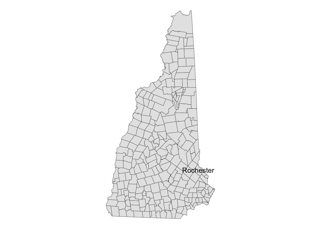

Land-use data

Land-use raster data come from the Multi-Resolution Land Characteristics (MRLC) Consortium. These data offer 30-m resolution (wow!) for the entirety of the continental US. but, Professor K has limited these data to an area covering NH. These data are available for download from our class site.

Let’s load the data and then create another object, lu2, that sets the attribute name to “land_use”, transforms the coordinate system and extent of the data to that of the nh sf object, and finally, downsamples the data 30 times, making each pixel 30 times larger. This last operation, using st_downsample() makes the resolution much more coarse, but eminently more manageable in terms of size and time to work with. Ah, tradeoffs. This could take a while, but it’s worth it in the end.

#large data set, 30m resolution
lu <- stars::read_stars("data/land_use/NLCD_2021_Land_Cover_L48_20230630_qtPZ6zMaTAibmibqfd37.tiff")

lu2 <- lu %>% 
 setNames("land_use") %>% 
     st_transform( st_crs(nh)) %>% 
  st_downsample(30,mean) %>% 
  st_crop(nh)  #lower res for plotting and handling

## Warning in st_crop.stars(., nh): crop only crops regular grids

Next steps

You’re tasked with combining all three data sets to undertake a random forest analysis. Here are some hints and requirements:

Use left_join() to join the deer object to the nh sf object. Please save this joined object as nh_deer and keep only the TOWN and HSM in addition to the geometry.
Create an object named nh_lu that is the result of a spatial join of the nh object to the lu2 object. Keep only land_use, TOWN, and the geometry.
Create an object named nh_dat that contains the relative proportion of land use and HSM for each town. Hint: dplyr::group_by(..., .drop = FALSE) and dplyr::count() should help in establish counts, including 0’s, on a per-Town basis.
Based on nh_dat, create an object named rf_dat that contains only the data needed to run an RF model that predicts HSM based on land-use patterns. Note: please arcsine transform your proportions data, a standard practice.

Project Report

Please submit your report to your team GitHub repository as an .Rmd document with HTML output that addresses the following questions:

Is WTD abundance spatially autocorellated, that is visually, are there pockets of higher or lower WTD harvest?
- In answering this question, please produce a pretty, interactive map.
Does land-use pattern predict WTD harvest values?
- Please establish a data tibble based on joining and intersecting the three data sources as outlined above.
- Using a tuned random forest model, assess whether land-use proportion in each town predicts deer-harvest values and which land-use pattern is important in this prediction.

In answering these questions, be sure to use the visualization, modeling, and model-assessments tools we’ve used in the course so far.

The answers and narrative in your .Rmd should include the following components:

A YAML header that specifies HTML output, the authors, and a bibliography named “BIOL3140.bib”. Submit this bibliography as well!
Sections including an introduction, methods, results, discussion, author contributions, and references. Make sure that each, aside from the references, includes one to two short paragraphs. Specifically:
- Introduction: Frame the questions, indicating why they are important, what background work has been done in this realm, and how you will answer them. Please include at least one reference to support the summary of previous work. Note: this can be done easily by refiguring the introduction to this project report.
- Methods: Explicitly state how you answered the questions, including a narrative of all the analyses both qualitative and quantitative.
- Results: Include any appropriate figures or tables and a narrative of the main results that are important to answering the questions.
- Discussion: Succinctly declare how the results relate to the question and how they compare to previous work devoted to the topic. In addition, be sure to comment on the importance of your findings to the broader topic at hand. Please include at least one reference to another relevant study. Note: circling back to the introductions, both to this project description and yours, will be helpful here.
- Author contributions: Briefly outline what each team member contributed to the project.

Project reports should be uploaded by 11:59 PM on Sunday, November 10th.

Please have a look at out Phase II report rubric to get a sense of how this and other Phase II reports will be grade.

Module 6 Project